While working with some sonar data, I found myself wanting to index a data file. I needed a key-value map where both the keys and the values are 64 bit integers. The values are essentially offsets into the original data file, but the keys are the concatenation of three integer fields from the data record itself. The first byte is the sonar subsystem that the data originated from, the next six bytes are a millisecond-resolution timestamp, and the final byte distinguishes the port from the starboard channel. I organize the keys this way because I have found that a lot of data access patterns require accessing the two channels of data from each timestamp for a particular subsystem. To scan the index in this way, we need to be able to iterate over keys that share a common prefix. A trie is a natural fit for this problem.

Tries are trees where the nodes represent common prefixes of the keys, and the edges represent the next symbol in the key. With integer keys, we can interpret the key as a string of bits, so that a very simple trie node consists of two pointers, one of which points to the subtrie where the prefix of the present node is followed by a 0 bit and one of which points to the subtrie where the prefix is followed by a 1 bit. In C, this might look something like

 typedef  struct  trie  trie;
 struct  trie {
     trie * children[2];
};

A 64 bit integer key can be found in the trie by scanning from the root node, which represents the empty prefix, and following 64 pointers by consuming bits from the key starting from the most significant bit. If we ever hit a NULL pointer, the key is not present, and we break out from the loop early. We don't need to store the keys in the trie, because they are implicitly represented by the path from the root node.

 trie * trie_lookup( trie * t,  uint64_t  key)
{
     for ( int32_t  level = 63; level >=0; level--) {
         uint8_t  child = (key >> level) & 1;
         if ( !t->children[child]) {
             return  NULL;
        }
        t = t->children[(key >> level) & 1];
    }
     return t;
}

trie_lookup returns a pointer to a trie, and a NULL pointer indicates that the key was not found. Note that this requires that the child pointers at level 0 are non-zero. They don't necessarily need to point to a valid trie, if we can ensure that we never dereference the pointer returned from trie_lookup. However, it is helpful when we start storing values in the trie to instead allocate a leaf node at a fictitious level equivalent to -1, so that the level 0 child pointers are either NULL or valid pointers to leaf nodes. Insertion is very similar to lookup.

 trie * new_node();
 trie * trie_insert( trie * t,  uint64_t  key)
{
     for ( int32_t  level = 64; level>=0; level--) {
         uint8_t  child = (key >> level) & 1;
         if ( !t->children[child]) {
            t->children[child] = new_node();
        }
        t = t->children[child];
    }
}

The function new_node depends on your chosen strategy for memory allocation. One could simply use malloc(sizeof(trie)), but I would usually allocate from a pool of trie nodes or a linear allocator. A simple pool allocator is just a buffer of trie nodes that tracks the next available node.

 typedef  struct {
     trie*  buffer;
     ptrdiff_t  capacity;
     ptrdiff_t  count;
}  trie_pool;

 trie * pool_allocate( trie_pool * pool)
{
    assert(pool->count < pool->capacity);
     return pool->buffer[pool->count++];
}

Before considering how to iterate over a trie, we can store values in the trie by changing the trie to a union.

 typedef  union  trie  trie;
 union  trie {
     trie * children[2];
     struct {
         uint64_t  key;
         uint64_t  value;
    };
};

The nodes on the fictitious -1 level will be leaf nodes with key-value pairs stored instead of child pointers. Rather than tagging the union, we will distinguish the internal from the leaf nodes by their level, which we will always keep track of outside of the data structure. While we don't need to store the keys, there is a spare 8 bytes in the leaf nodes that we might as well fill up, and storing the keys prevents us from having to keep track of the keys while iterating.

Our trie is a binary tree and iterating over it amounts to a depth-first tree traversal, which means we need a stack.

 typedef  struct {
     trie * stack[65];
     int32_t  levels[65];
     int32_t  top;
}  trie_iterator;

 void  trie_push( trie_iterator * iter,  trie * node,  int32_t  level)
{
    assert(iter->top < 65);
    iter->levels[iter->top] = level;
    iter->stack[iter->top++] = node;
}

 int32_t  trie_pop( trie * node,  trie_iterator * iter)
{
    assert(iter->top > 0);
    node = iter->stack[--iter->top];
     return iter->levels[iter->top];
}

The trie has a fixed depth, so the stack is bounded by the number of levels, which is 64 plus the leaf level, so 65 nodes will suffice. We maintain a stack of trie pointers and their corresponding levels. If we didn't store the keys in the leaves, we would also want to have a stack of keys, which we would reconstruct as we progress through the trie.

We initialize the iterator by pushing the root node at level 63:

 trie_iterator  trie_begin( trie * root)
{
     trie_iterator  iter = {0}; 
    trie_push(&iter,root,63);
     return iter;
}

To iterate, we pop nodes from the stack and push their children.

 trie * trie_iterate( trie_iterator * iter,  int32_t  end_level)
{
     trie * node;
     int32_t  level;
     while (iter->top > 0) {
        level = trie_pop(node,iter);
         if (level < end_level) {
             return node;
        }
         if (node->children[1]) {
            trie_push(iter,node->children[1],level - 1);
        }
         if (node->children[0]) {
            trie_push(iter,node->children[0],level - 1);
        }
    }
     return  NULL;
}

We use the end_level parameter to control which nodes we iterate over. If we want to iterate over the leaf nodes, we pass 0 for end_level. If we want to iterate over prefixes, we pass end_level corresponding to the level of the prefix. For our sonar data example, we might iterate first over the subsystems, then over the timestamps, then the channels.

 trie_iterator  subsystem_iterator = trie_begin(root);
 trie * subsystem;
 while ((subsystem = trie_iterate(&subsystem_iterator,56))) {
     trie_iterator  timestamp_iterator;
    trie_push(×tamp_iterator,subsystem,55);
     trie * timestamp;
     while ((timestamp = trie_iterate(&subsystem_iterator,8))) {
         trie_iterator  channel_iterator;
        trie_push(&channel_iterator,timestamp,7);
         trie * channel;
         while ((channel = trie_iterate(&channel_iterator,0))) {
            process_data(channel->key,channel->value);
        }
    }
}

And that is all we need to start building and scanning indices for the sonar data. There are a lot of improvements that we can make on this basic design. For example, we can consume more than a single bit of the key at a time, which speeds up lookups while requiring more space to store the child pointers. We can also construct a variety of hybrid tree variants that use other search data structures at each level of the trie. It is also relatively straightforward to implement lock-free concurrent inserts to this simple array-based trie.

I have just published a little command line tool called goneplax to help look at the JSF files that are output by Edgetech sonars. Imaging sonar data is an interesting problem because publicly accessible data usually is either georeferenced mosaics or raw instrument data. The former come in geospatial formats like GeoTIFFs but have lost a lot of information that I would like to have as I think about statistical models for imaging sonar data. The latter typically need proprietary software to access, and that software often locks you into particular kinds of data analysis like the production of georeferenced mosaics. There are some open source sonar data tools, notably MB-System from the Monterey Bay Aquarium Research Institute, but those aim to be fully featured data processing systems, whereas I am mostly interested in tools that allow me to build my own data analysis pipelines around sonar data.

However, my earlier attempt at this kind of tooling quickly ballooned out of control because there is a lot of stuff you can do with sonar data like format translation, visualization or even data analysis tools – I even briefly messed around with designing a programming language. I took a step back, thought about The Joy of Small Projects, and this morning came up with goneplax. I have a lot of JSF files sitting around (two particularly good sources for sonar data are PANGAEA and the UK government data portal), and the first step to using them for anything is to figure out what is in them. JSF files are basically sequences of records, each of which has a header that provides some information about the record. goneplax reads through these records, and writes out to the command line the type of each record, the subsystem it comes from and the channel within that subsystem (i.e. the port or starboard channels for sidescan data).

If we try it out on some data from Papenmeier and Hass (2019), we get something like

> goneplax HE501_Hydro1_001.jsf | head
System Information:0:0
Navigation Offsets:0:0
Pitch Roll Data:101:1
Pitch Roll Data:101:1
Sonar Data Message:20:0
Sonar Data Message:20:1
Pitch Roll Data:101:1
Unknown Message:102:0
Pitch Roll Data:101:1
Sonar Data Message:20:0

The first field is the type of the message, the second is the subsystem number and the third is the channel. For instance, in the first 10 records shown above, we have three Sonar Data Messages that contain sidescan data. These are all from subsystem 20, which is the code for the lowest available sidescan sonar frequency (these data only have one frequency). The first and the last are from the port side of the sonar (channel 0) and the second is from the starboard (channel 1).

goneplax outputs text data like this so we can use Unix command line tools to further process it. One common operation is to count the number of messages of each kind in a given file:

> goneplax HE501_Hydro1_001.jsf | sort | uniq -c
    1 Navigation Offsets:0:0
 9370 NMEA String:100:0
19440 Pitch Roll Data:101:1
 8721 Sonar Data Message:20:0
 8720 Sonar Data Message:20:1
    1 System Information:0:0
 1500 Unknown Message:102:0

which matches the output of jsfmesgtype, another command line tool that does something similar:

> jsfmesgtype HE501_Hydro1_001.jsf
Sonar = 17441  Pitch = 19440  NMEA = 9370  Analog = 1500  S_info = 1

If goneplax seems like it might be useful for you, give it a try and let me know how it goes at ~wkearn/goneplax-discuss@lists.sr.ht.

Gaussian processes are powerful tools for modeling spatially varying fields like sea surface temperature or sand ripple elevation. But what can you do if you want a model for discrete-valued fields like a land cover classification? There are many approaches that you could use for this problem, but I particularly like the maps you can generate using spatially dependent Pitman-Yor processes ( Sudderth and Jordan 2008).

A Pitman-Yor process is a generalization of the Dirichlet process. Both are probability distributions over probability distributions in a sense that is quite tricky to understand, but which is very useful in developing nonparametric Bayesian models for data: you can use a Dirichlet/Pitman-Yor prior for an unknown probability distribution and then learn the distribution from your data.

Another way of looking at these processes is that they provide distributions over infinite partitions of the interval \([0,1]\). This is often called the "stick-breaking" construction of the Dirichlet process, and it works like this. Imagine we have a stick with a unit length. We first break off a randomly sized fraction of the stick, \(v_1\). This is the first segment of our partition with length \(p_1 = v_1\). Now we take the remaining stick, which has a length \(1 - v_1\), and we break off another piece that is a fraction, \(v_2\), of the remaining length. This piece is our second segment, and it has a length of \(p_2 = v_2 (1 - v_1)\). We repeat this process an infinite number of times, so that the $k$-th segment has a length \(p_k = v_k \prod_{i=1}^{k-1} (1 - v_k)\), and the segments all add up to the length of the original stick \(\sum_{k=1}^{\infty} p_k = 1\).

The difference between the Dirichlet process and the Pitman-Yor process is simply in the distribution of the fractions, \(v_k\). The Dirichlet process has each fraction distributed by a \(\text{Beta}(1,\alpha)\) distribution while the Pitman-Yor process has

\[ v_k \sim \text{Beta}(1 - \beta,\alpha + k \beta) \]

so that the distribution changes with \(k\). When \(\beta = 0\), this is just the Dirichlet process while higher values of \(\beta\) result in a distribution with heavier tails than the Dirichlet process.

For our Pitman-Yor process maps, we only need to sample the fractions, \(v_k\), which we can do easily in Julia using Distributions.jl to sample from the Beta distribution

 function  sample_py_fractions(α,β,K)
  v = zeros(K)
   for k  in 1:K
      v[k] = rand(Beta(1 - β, α + k * β))
   end
  v
 end

Note that even though the partition formally has an infinite number of segments, we only sample the first \(K\) fractions. One interpretation of the Dirichlet process is as a mixture model with an infinite number of components. The partition lengths, \(p_k\), are the relative frequencies of each class: \(p_1\) percent of your data will come from class 1, \(p_2\) come from class 2, and so on. Since \(p_k\) is always smaller than \(p_{k-1}\), only a finite number of classes will have a meaningful probability of being drawn, even though the model theoretically represents an infinite number of classes. As long as \(K\) is high enough that we don't hit that threshold, it is okay to only think about the first \(K\) classes.

In this classification model, it turns out that the stick-breaking fraction \(v_k\) is the conditional probability of assigning a data point to class \(k\) given that all the classes with indices less that \(k\) have been rejected. So we can think about generating class assignments by first choosing class 1 with probability \(v_1\). If we don't choose class one then we choose class 2 with probability \(v_2\), and so on, until all of our data points are assigned to classes. In code, this process looks something like

 function  generate_classes(v,N)
    z = zeros(Int,N)
     for i  in 1:N
        k = 1
         while (k <= length(v)) && (rand() > v[k])
            k += 1
         end
        z[i] = k
     end
    z
 end

The insight that allows Sudderth and Jordan to create spatially dependent Pitman-Yor processes is that instead of drawing uniform random variables and checking whether they are less than the stick-breaking fraction, we can draw random variables from a different distribution, apply the cumulative distribution function for that distribution to the random variable and compare that value to the stick-breaking fraction. This is the same idea behind inverse transform sampling, which lets you convert uniformly distributed random variables into arbitrarily distributed variables provided that you know the (inverse) cumulative distribution function.

In particular, we can choose standard normal random variables and apply the CDF of the normal distribution to sample from the same distribution of classes. Furthermore, instead of drawing independent samples, they can have correlations across the data points, as long as the marginal distributions are standard normal. It is important to note that the correlations are across data points (the index \(i\) in the above code) not the classes. Those still need to be independent to get the class proportions correct.

Gaussian processes are just normally distributed random variables with spatial correlations, so we can build spatially dependent Pitman-Yor processes by first drawing \(K\) independent realizations of Gaussian processes over our region of interest, drawing stick-breaking fractions as above, and then applying our classification scheme for each point in space.

There are a lot of details to sampling from Gaussian processes, so we won't look into them in great detail here. Instead we will just use the following function that generates random fields on regular grids using fast Fourier transforms.

 function  generate_field(k0,ν,Nx,Ny,B)
  kx = FFTW.rfftfreq(Nx)
  ky = FFTW.fftfreq(Ny)
  k2 = abs2.(kx) .+ abs2.(ky')
  v = inv(sqrt(π/ν)) * (k0^ν) .* (abs2(k0) .+ k2).^(-(ν+1)/2)
  irfft(v .* rfft(randn(Nx,Ny,B),(1,2)),Nx,(1,2))
 end

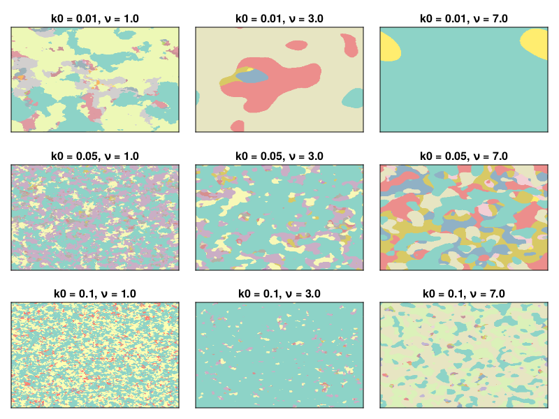
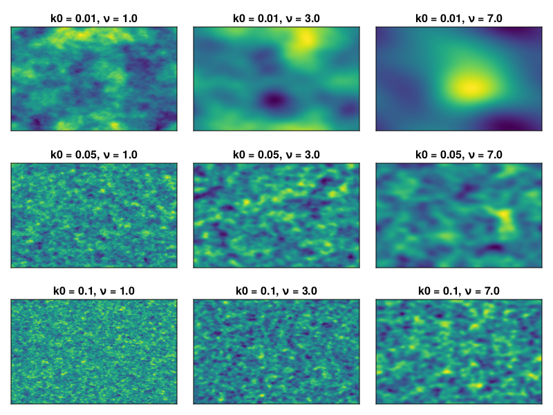
The parameter \(k_0\) sets the correlation length of the field: higher \(k_0\) corresponds to shorter correlation lengths, and the parameter \(\nu\) controls the smoothness of the field, with higher \(\nu\) giving smoother fields. The following figure illustrates some random fields as shown in the following figure

k0 = [0.01;0.05;0.1]
ν  = [1.0;3.0;7.0]

fields = [generate_field(k0,ν,256,256,1)[:,:,1]  for k0 in k0, ν  in ν]
fig = Figure()
 for j  in 1:3
     for i  in 1:3
        ax = Axis(fig[i,j],title= "k0 = $(k0[i]), ν = $(ν[j])")
        heatmap!(ax,fields[i,j])
        hidedecorations!(ax)
     end
 end

save( "patchwork-fields.png",fig)

Finally we just need to modify generate_classes so that it uses the random fields as input to generate the classes.

 Φi(v) = -erfcinv(2v) * sqrt(2)
 function  classify_fields(u,v)
  z = zeros(Int,size(u,1),size(u,2))
   for j  in 1:size(u,2)
       for i  in 1:size(u,1)
          acc =  false
          k = 1
           while (k < size(u,3)) && (u[i,j,k] >= Φi(v[k]))
              k += 1
           end
          z[i,j] = k
       end
   end
  z
 end

Note that we defined the function Φi(v) which is the inverse of the standard normal cumulative distribution function.

We can wrap all of this together in a function to generate a map

 function  generate_map(α,β,k0,ν,Nx,Ny,K)
    v = sample_py_fractions(α,β,K)
    u = generate_field(k0,ν,Nx,Ny,K)
    classify_fields(u,v)
 end

and make some maps

k0 = [0.01;0.05;0.1]
ν  = [1.0;3.0;7.0]

maps = [generate_map(1.0,0.0,k0,ν,256,256,32)  for k0 in k0, ν  in ν]

fig = Figure()
 for j  in 1:3
     for i  in 1:3
        ax = Axis(fig[i,j],title= "k0 = $(k0[i]), ν = $(ν[j])")
        heatmap!(ax,maps[i,j],colormap= :Set3_12)
        hidedecorations!(ax)
     end
 end

save( "patchwork-maps.png",fig)

The (cubic) smoothing spline is usually introduced as a minimization problem: find the function, \(f\) that minimizes the following functional

\[ J(f) = \sum_{i=1}^N (y_i - f(x_i))^2 + \lambda\int f''(x)^2\,dx \]

that balances fitting the data in the first term and the smoothness of the chosen function in the second, with the tradeoff determined by the smoothing parameter \(\lambda\). ¹ It turns out that the solution to this minimization is a piecewise cubic polynomial with knots at the data locations. Fitting this function is straightforward but requires some careful application of linear algebra to be efficient (Reinsch).

When the data are measured at regular intervals, such as in many time series applications, the integral can be replaced by the discrete sum

\[ \sum_{t=2}^{N-1} \left(f_{t+1} - 2f_t + f_{t-1}\right)^2. \]

where \(f_t = f(x_t)\) is the value of the unknown function at each of the data points. Our modified objective function now reads

\[ J(f_{1:t}) = \sum_{t=1}^N (y_t - f_t)^2 + \lambda \sum_{t=2}^{N-1} \left(f_{t+1} - 2f_t + f_{t-1}\right)^2 \]

and one way to interpret this optimization problem is as minimizing the sum of squares of the residuals, \(w_t\) and \(v_t\) in

In fact, this pair of equations defines a state-space model, which means we can use Kalman filtering and smoothing techniques ^{2 , 3} to estimate the posterior mean \(E[f_{1:t}|y_{1:t}]\), which turns out to coincide with the smoothing spline solution. The one tricky point is that standard Kalman smoother implementations require you to specify an initial distribution for \(f_{-1:0}\). The Kalman smoother and the smoothing spline only coincide when this prior distribution becomes very diffuse. This is because the smoothing spline is technically equivalent to an "improper" Bayesian prior on \(f_{1:t}\). ^{1 , 4}

Reframing the smoothing spline algorithm to a generative model for some data makes it possible to build smoothing splines into more complex models. One could, for example, combine the smoothing spline prior with a non-Gaussian likelihood to model count or classification data.

In my last post I speculated on the usefulness of probabilistic programming in geographic information systems (GIS). While I have played with some probabilistic programming languages (PPLs) like Turing, I mostly do statistical inference using my own code, specialized for the particular models I am trying to build. I wanted to learn more about how PPLs work to start thinking harder about how one might build a GIS around one. It turns out that it is not that hard to get a very rudimentary PPL up and running, so I thought I would share how I did that in (more or less) 100 lines of Julia code.

 using Distributions, LinearAlgebra, Statistics, CairoMakie, Random
Random.seed!(54332187)

 struct  LatentDistribution
    f
    s
    d
 end

model = LatentDistribution(X-> nothing, :X,Normal(0,1))

model = LatentDistribution( :X,Normal(0,1))  do X
     nothing
 end

model = LatentDistribution( :X,Normal(0,1))  do X
    LatentDistribution( :Y,Normal(X,1))  do Y
         #  We don't need to explicitly return nothing
     end
 end

 function  draw(d:: LatentDistribution)
     #  Sample from the given distribution
    x = rand(d.d)

     #  Call the continuation with the sampled value
     #  and draw from that distribution
    draw(d.f(x)) 
 end

 draw(:: Nothing) =  nothing

 function  draw(d:: LatentDistribution)
     #  Sample from the given distribution
    x = rand(d.d)

    (;d.s => x,  #  Store the sampled value
     draw(d.f(x))...)  #  Recurse
 end

 draw(:: Nothing) = (;)  #  Return an empty named tuple

(x = -0.2817850808916265, y = 0.6312531437930013)

 function Distributions. logpdf(d:: LatentDistribution,θ)
     #  Extract the variable corresponding to the current
     #  distribution
    x = θ[d.s]

     #  Compute the logpdf of the current variable
    logpdf(d.d,x) +
         #  Recurse
        logpdf(d.f(x),θ)
 end
Distributions. logpdf(:: Nothing,θ) = 0  #  Start accumulating probability from 0

 struct  ObservedDistribution
    f
    s
    d
    y
 end

 function  draw(d:: ObservedDistribution)
    y = d.y
    (;d.s=>y,draw(d.f(y))...)
 end
 function Distributions. logpdf(d:: ObservedDistribution,θ)
    loglikelihood(d.d,d.y) + logpdf(d.f(d.y),θ)
 end

model = LatentDistribution( :X,Normal(0,1.0))  do X
    ObservedDistribution( :Y,Normal(X,1.0),[1.0;-0.2;0.3])  do Y
     end
 end

proposals = Dict( :X => θ -> Normal(θ.X,0.01))

proposals = Dict( :X => θ -> Normal(1/(1 + length(θ.Y)) * sum(θ.Y),inv(sqrt(1 + length(θ.Y)))))

 gibbs(:: Nothing,θ,proposals) = θ
 gibbs(d:: ObservedDistribution,θ,proposals) = gibbs(d.f(d.y),θ,proposals)

 function  gibbs(d:: LatentDistribution,θ,proposals)
     #  Extract the current variable
    x = θ[d.s]

     #  Construct the proposal distribution
    q = proposals[d.s](θ)

     #  Sample from the proposal distribution
    x′ = rand(q)
    θ′ = (;θ...,d.s=>x′)

     #  Construct the reversed proposal
    q′ = proposals[d.s](θ′)

     #  Compute the log acceptance ratio
    α = logpdf(d,θ′) + logpdf(q′,x) - logpdf(d,θ) - logpdf(q,x′)

     #  Rejection sampling
     if log(rand()) < α
         #  Accept the proposal
         #  and recurse
         return gibbs(d.f(x′),θ′,proposals)
     else
         #  Reject the proposal
         #  and recurse
         return gibbs(d.f(x),θ,proposals)
     end
 end

Example

As an example, we will fit the following Bayesian linear regression to some synthetic data

\begin{align} \beta &\sim \mathcal{N}(0,I) \\ \tau &\sim \Gamma(2,1) \\ Y | X,\beta,\tau &\sim \mathcal{N}(X\beta,\tau^{-1}) \end{align}

 #  Generate some synthetic data
N = 100
x = range(-1,1,length=N)
X = [one.(x) x]
β0 = [1.0;-1.0]
σ0 = 1.0

Y = X * β0 .+ σ0 * randn(N)

 #  Define the model
model = LatentDistribution( :β,MvNormal(Diagonal(ones(2))))  do β
    LatentDistribution( :τ,Gamma(2,1))  do τ
        ObservedDistribution( :Y,MvNormal(X*β,inv(sqrt(τ))),Y)  do Y
         end
     end
 end

 #  Define the proposal distributions
proposals = Dict( :β => θ -> MvNormalCanon(θ.τ*X'θ.Y,θ.τ*X'X+I),
                  :τ => θ -> Gamma(2 + length(Y)/2,inv(1 + sum(abs2,θ.Y .- X*θ.β)/2)))

 #  Draw an initial value from the model
θ0 = draw(model)

 #  Run 100000 Gibbs steps
θs = accumulate((θ,i)->gibbs(model,θ,proposals),1:100000,init=θ0)

βs = mapreduce(x->x.β,hcat,θs)
τs = map(x->x.τ,θs)

 #  Plot the results
fig = Figure()
ax1 = Axis(fig[1,1],xlabel= "x",ylabel= "Y")
scatter!(ax1,x,Y)
ax2 = Axis(fig[2,1],xlabel= "β")
density!(ax2,βs[1,:])
density!(ax2,βs[2,:])
vlines!(ax2,[β0[1]])
vlines!(ax2,[β0[2]])
ax3 = Axis(fig[3,1],xlabel= "τ")
density!(ax3,τs)
vlines!(ax3,[inv(σ0^2)])
save( "linear_regression.png",fig)

Luke Bergmann and Nick Lally, in their article "For geographical imagination systems" ( paywalled link, pdf via Nick Lally), state that

knowledge that was once entwined with particular knowers and communities and contexts is first alienated into separate data layers, then those layers are then reintegrated by GISystems according to common location.

(Bergmann and Lally, p. 8)

As a result, GIS are built around some absolute coordinate system to which all data must be referenced before we can analyze them or create visualizations. GIS in this paradigm are essentially UI wrappers around libraries like PROJ and GDAL that convert data from different coordinate systems and formats into a common reference frame. Information that doesn't fit neatly into a coordinate either needs to be forced into the GIS or discarded altogether.

Bergmann and Lally present a prototype "geographical imagination system" enfolding that challenges this paradigm by building visualizations of geographic information using non-Euclidean distance metrics that highlight relations between phenomena that coexist with traditional spatial relations. I think they are mostly interested addressing challenges that arise with GIS in human geography, but their articulation of these limitations of GIS illuminates some of the difficulties I have encountered in dealing with geospatial data in the geosciences. Earth observations are noisy, incomplete windows into the world. When we try to build and test models using these data, we need to be aware of how our inferences might be affected by the circumstances of their acquisition and processing. Our GIS generally don't make this easy for us. But they could.

One possibility that I have been thinking about recently is replacing the GIS notion of data layers with a probabilistic graphical model (PGM) in which data is represented by a collection of vertices that represent the different quantities of interest, including both observed and unobserved, and edges that encode hypothesized probabilistic relationships between quantities. Some of those quantities might be spatial coordinates associated with a particular object, but every quantity need not have a spatial representation. Multiple spatial representations can coexist, with deterministic coordinate transformations replaced by probabilistic mappings. Because everything is framed as a PGM, it could be written in a probabilistic programming language to facilitate automatic statistical inference, uncertainty quantification and model validation and comparison.

I would really like GIS software that centers model building as an interpretive tool, and I think this PGM approach has some potential to do that. Different researchers working with the same data may embed them in different models, so that a dataset need not have a single, fixed meaning. Visualization, which often seems to be the central focus of GIS, becomes a tool to inspect the performance of models and encompasses a much wider range of data visualizations than cartographic ones. A major challenge, I think, is in designing software that allows users to gradually integrate these modeling ideas into their workflow.

One problem I have been interested in recently is numerical methods for computational fluid dynamics in semi-infinite domains, where you have some kind of boundary at \(z=0\), and the domain extends upwards to infinity. This is quite relevant to bottom boundary layer simulations, which typically impose artificial boundary conditions at some large \(z\) value. If you could simulate the problem on the infinite domain, then you can avoid having to worry about whether those artificial boundary conditions are influencing your solution. A model problem that is useful for evaluating numerical methods in these situations is the forced diffusion equation

\[ \frac{\partial u}{\partial t} = \frac{\partial^2 u}{\partial z^2} + \cos(t) \]

with a homogeneous boundary condition \(u(z=0,t) = 0\). This problem ("Stokes problem") arises when considering a laminar boundary layer driven by an oscillating pressure gradient, and it is useful because it has an analytical solution

\[ u(z,t) = \sin(t) - e^{-\frac{z}{\sqrt{2}}} \sin\left(t - \frac{z}{\sqrt{2}}\right) \]

to which we can compare our numerical solutions.

To work with the infinite domain, we apply a coordinate transformation ( Boyd 2000)

\[ s = \frac{z - 1}{z + 1} \]

of the interval \(\left[0,\infty\right)\) to \([-1,1)\). This coordinate transformation turns the \(z\) derivative into an \(s\) derivative multiplied by a quadratic polynomial.

\[ \frac{\partial u}{\partial z} = \frac{\left(1 - s\right)^2}{2} \frac{\partial u}{\partial s} \].

The forced diffusion equation in the new coordinates is

\[ \frac{\partial u}{\partial t} = \frac{\left(1 - s\right)^2}{2} \frac{\partial}{\partial s}\left(\frac{\left(1 - s\right)^2}{2} \frac{\partial u}{\partial s}\right) + \cos(t) \]

with the boundary condition \(u(s=-1,t) = 0\). Since we are now working on the interval \(s \in [-1,1)\), it makes sense to represent \(u\) using an expansion in Chebyshev polynomials.

\[ u(s,t) = \sum_{k=0}^\infty u_k(t)T_k(s) \]

The diffusion equation becomes

\[ \frac{\partial \mathbf{u}}{\partial t} = L \mathbf{u} + F(t) \]

where \(\mathbf{u} = [u_0,u_1,\dots]\) is the vector of Chebyshev coefficients, \(L\) is the matrix representing the action of the second derivative operator on the Chebyshev coefficients. We need to supplement this with the boundary condition, \(\sum_{k=0}^{\infty} (-1)^k u_k = 0\).

The matrix \(L\) can be derived from the recurrence relationships for Chebyshev polynomials. It takes the form \(L = GDGD\) where

\[ D = \begin{bmatrix} 0 & 1 & 0 & 3 & 0 & 5 & \dots \\ 0 & 0 & 4 & 0 & 8 & 0 & \dots \\ 0 & 0 & 0 & 6 & 0 & 10 & \dots \\ \vdots & \vdots & \vdots & \vdots & \vdots & \vdots & \vdots\\ 0 & 0 & 0 & 0 & 0 & 0 & \dots \\ \end{bmatrix} \]

is the derivative operator and \(G\) represents multiplication by \(g(s) = \frac{1}{2}\left(1 - s\right)^2\). Since that function is a quadratic polynomial, it can be represented by a three term Chebyshev series \(g(s) = \frac{3}{4}T_0(s) - T_1(s) + \frac{1}{4}T_2(s)\), which, because of the recurrence relations of Chebyshev polynomials, means that the matrix \(G\) is a banded matrix ( Olver and Townsend 2013, p. 7)

\[ G = \begin{bmatrix} \frac{3}{4} & -\frac{1}{2} & \frac{1}{8} & 0 & 0 & 0 & \dots \\ -1 & \frac{7}{8} & -\frac{1}{2} & \frac{1}{8} & 0 & 0 & \dots \\ \frac{1}{4} & -\frac{1}{2} & \frac{3}{4} & -\frac{1}{2} & \frac{1}{8} & 0 & \dots \\ \vdots & \vdots & \vdots & \vdots & \vdots & \vdots & \vdots\\ \end{bmatrix} \].

I've written these operators as infinite dimensional ones, but in practice, we truncate the Chebyshev expansion of \(u\) at \(N\) terms, which means we take the first \(N \times N\) block of the infinite dimensional matrix \(L\). Note that if we instead truncate \(G\) and \(D\) by taking the first \(N \times N\) blocks, we will end up with some additional error from the truncation of \(G\). Since we know \(G\) and \(D\) analytically, it is easy enough to work out the operator \(L\) by truncating the operators at some \(M > N\) and then taking the first block of \(L\). For this particular application \(M = N + 1\) is enough to avoid additional truncation errors.

While \(G\) is banded, \(D\) is essentially dense, and the operator \(L = GDGD\) is dense. We can get sufficient numerical results using this operator, but solving the dense linear system \(L\mathbf{u} = b\), as we need to do when we implicitly discretize time, scales as \(\mathcal{O}(N^2)\) when we precompute the LU decomposition of \(L\). This quadratic scaling is problematic when we need to apply this solver many times such as when we are timestepping the diffusion equation.

We can, however, do better using the ultraspherical method of Olver and Townsend (2013). This rests on the fact that the derivatives of Chebyshev polynomials are scaled ultraspherical polynomials. Since we need two derivatives, we can convert to the ultraspherical basis of order 2 using the conversion matrices given on p. 8 and p. 12 of Olver and Townsend. This renders the second derivative matrix \(D^2\) diagonal and the operator \(L = S_1S_0GDGD\) banded. Because it is banded, solving the linear system only requires \(\mathcal{O}(N)\) operations at each time step.

 using LinearAlgebra, SparseArrays

 function  chebyshev_derivative_matrix(Nz)
    sparse([(i < j)  ? (i==0 ? 1 : 2)*j*mod(i+j,2)  : 0  for i in 0:Nz-1, j  in 0:Nz-1])
 end

 function  chebyshev_multiplication_matrix(Nz)
    G0 = sparse([((i == j+0) + (i == abs(j-0)))//2  for i in 0:Nz-1, j  in 0:Nz-1])
    G1 = sparse([((i == j+1) + (i == abs(j-1)))//2  for i in 0:Nz-1, j  in 0:Nz-1])
    G2 = sparse([((i == j+2) + (i == abs(j-2)))//2  for i in 0:Nz-1, j  in 0:Nz-1])

     #  0.5 * (1 - s)^2 = 3//4 T₀ - T₁ + 1//4 T₂
    3//4 * G0 - G1 + 1//4*G2
 end

 S1(Nz) = spdiagm(0=>[1;[1//(1+k)  for k in 1:Nz-1]],2 =>[-1//(1 + k)  for k  in 2:Nz-1])
 S0(Nz) = spdiagm(0=>[2;ones(Int,Nz-1)] .// 2,2=>-ones(Int,Nz-2).//2)

 function  assemble_matrices(Nz,Δt,ultraspherical)
     #  Bottom boundary condition
    BC = [(-1)^k  for k  in 0:Nz-1]' 

     #  We make everything slightly larger to avoid truncation errors
    D = chebyshev_derivative_matrix(Nz + 1)
    G = chebyshev_multiplication_matrix(Nz + 1)
     if ultraspherical
        Δ = S1(Nz+1)*S0(Nz+1) * G*D*G*D
        A = S1(Nz+1)*S0(Nz+1) - Δt/2 * Δ
        B = S1(Nz+1)*S0(Nz+1) + Δt/2 * Δ
     else
         #  Assemble the Chebyshev matrices without
         #  the ultraspherical conversion
        Δ = G*D*G*D
        A = I - Δt/2 * Δ
        B = I + Δt/2 * Δ
     end


     #  Apply boundary bordering and truncate properly
    [BC;A[1:Nz-1,1:Nz]],B[1:Nz,1:Nz]
 end

 function  timestep!(un,u,A,B,Δt,t)
    RHS = B*u
    RHS[1] += Δt/12 * (23 * cos(t) - 16 * cos(t - Δt) + 5 * cos(t - 2Δt))

    RHS[ end] = 0
    circshift!(RHS,-1)
    ldiv!(un,A,RHS)
 end

 function  run_model(U0,A,B,Δt,Nt)
    U = zeros(length(U0),Nt+1)
    U[:,1] = U0
     for i  in 1:Nt
        timestep!(view(U,:,i+1),view(U,:,i),A,B,Δt,(i-1)*Δt)
     end
    U
 end

 function  stokes(z,t)
    sin(t) - exp(-z/sqrt(2))*sin(t - z/sqrt(2))
 end

 function  chebyshev_matrix(x,P=length(x))
    N = length(x)
    T = zeros(N,P)
    T[:,1] .= 1
    T[:,2] .= x
    T[:,3] .= 2x.^2 .- 1
     for i  in 3:P-1
        T[:,i+1] = 2*x.*T[:,i] .- T[:,i-1]
     end
    T
 end

 function  quadrature_error(z,u,u0)
    N = length(u)
    s = (z .- 1) ./ (z .+ 1)

    f = abs2.(u .- u0) .* sqrt.(1 .- s.^2)

    π*sum(f)/N
 end

 function  run_test(Nz,Δt,Nt,Nq=1024;ultraspherical= true)

     #  Chebyshev roots grid and transformed grid
     #  Note that we use a high resolution grid here
    s = [cospi((2k + 1)/2Nq)  for k  in 0:Nq-1]
    z = (1 .+ s) ./ (1 .- s)

    T = chebyshev_matrix(s,Nq)

     #  Initial conditions
    u0 = stokes.(z,0.0)
     #  Forward Chebyshev transform to compute coefficients
     #  Truncate from the high-order approximation
    U0 = (T\u0)[1:Nz]

    A,B = assemble_matrices(Nz,Δt,ultraspherical)
    Al = lu(A)

     #  Run once to compute the results
    U = run_model(U0,Al,B,Δt,Nt)

     #  Run again to time the solver
    t =  @elapsed run_model(U0,Al,B,Δt,Nt)

    u = T[:,1:Nz]*U
    err = [quadrature_error(z,u[:,i],stokes.(z,(i-1)*Δt))  for i  in 1:size(u,2)]
    u,t,err
 end

Results

If we run the model with Nz = 128 and Δt = 2π*0.01 for a single cycle, our results look something like this

Nz = 128
Δt = 2π*0.01
Nt = 100
Nq = 1024

u1,t1,err1 = run_test(Nz,Δt,Nt,Nq)

s1 = [cospi((2k + 1)/2Nq)  for k  in 0:Nq-1]
z1 = (1 .+ s1) ./ (1 .- s1)

 using CairoMakie
tidx = Observable(1)

uo = lift(tidx)  do i
    u1[:,i]
 end

fig = Figure()
ax = Axis(fig[1,1],ylabel= "Height",xlabel= "Velocity")
lines!(ax,uo,z1,color= :black)
ylims!(ax,0,10)
xlims!(ax,-1.1,1.1)

record(fig,  "ultraspherical_diffusion.mp4", 1:size(u1,2);framerate=30)  do i
    tidx[] = i
 end

A video of a single period of the oscillating boundary layer flow

At this resolution, the numeric and analytic solutions are basically identical, so I have only plotted the numeric solution.

We can also run it at several resolutions to see how the computational time and the error scales with the grid size. We will run it for 10 cycles just to make sure that it is stable for long integration times. We will also run the Chebyshev method which results in dense matrices to compare its performance to the ultraspherical method.

Nzs = 16:16:256
res0 = [run_test(Nz,Δt,10*Nt,Nq;ultraspherical= false)  for Nz  in Nzs]
res1 = [run_test(Nz,Δt,10*Nt,Nq;ultraspherical= true)  for Nz  in Nzs]
us0,ts0,err0 = map(x->x[1],res0),map(x->x[2],res0),map(x->x[3][ end],res0)
us1,ts1,err1 = map(x->x[1],res1),map(x->x[2],res1),map(x->x[3][ end],res1)


fig2 = Figure()
ax1 = Axis(fig2[1,1],ylabel= "Time (s)",xlabel= "Grid size")
scatter!(ax1,Nzs,ts0,label= "Chebyshev",marker= :circle)
scatter!(ax1,Nzs,ts1,label= "Ultraspherical",marker= :diamond)

axislegend(ax1,position= :lt)
ax2 = Axis(fig2[2,1],ylabel= "Error",xlabel= "Grid size",yscale=log10)
scatter!(ax2,Nzs,err0,label= "Chebyshev",marker= :circle)
scatter!(ax2,Nzs,err1,label= "Ultraspherical",marker= :diamond)
axislegend(ax2,position= :rt)


save( "ultraspherical_scaling.png",fig2)

We can see that the ultraspherical method scales linearly with N while the Chebyshev method scales quadratically. The Chebyshev method has a lower error at small grid sizes, but the error converges between the two methods by N=64. At that point, most of the error is due to the time discretization, and it can be decreased further by decreasing the time step.

Spectral methods are really neat ways to solve PDEs accurately without a ton of effort, and the ultraspherical spectral method helps prevent the scaling issues that you get with a pure Chebyshev method. Using a coordinate transformation, it is also really easy to handle the semi-infinte domain that we want for theoretical bottom boundary layer studies. It is pretty straightforward to build an incompressible Navier-Stokes solver in this kind of framework, especially if we use periodic boundary conditions in the horizontal directions. The problem decouples into a set of vertical PDEs like our diffusion equation for each Fourier coefficient. One does have to address the incompressibility condition and the pressure computation, and we might see how that works later. Stay tuned!

You can find the Julia code contained in this file here.

Welcome to my personal website!

Subscribe to the Atom feed to keep up with additional updates.

Allison Penko and I just published a Naval Research Laboratory Technical Report about our seafloor evolution modeling framework. You can read the whole report at DTIC or arXiv.

The core model isn't new ( Traykovski (2007), Nelson and Voulgaris (2015), Penko et al. (2017)), but I've been working over the last few years on extending its capabilities, turning the Naval Seafloor Evolution Model (NSEM) into the Naval Seafloor Evolution Architecture (NSEA). We have replaced the original Fortran implementation with one written in Julia, which lets us easily do some cool things such as running NSEA on the GPU using GPUArrays.jl. I've also developed tools for statistical inference that use seafloor roughness observations to estimate sediment transport parameters like the sediment grain size and the critical shear stress.

I am especially proud of the section that draws out the connection between NSEM and a particular stochastic sediment flux model. NSEM doesn't model the actual transport of sediment and formation of bedforms. Instead, it uses some heuristics, scaling arguments and empirical parameterizations to model the evolution of the power spectrum of the seafloor roughness. This works surprisingly well when the seafloor roughness is predominantly small-scale ripples formed by wind waves, but it runs into trouble when you want to apply it to different settings like current-driven ripples or bedforms created by internal waves because those empirical parameterizations fail in these situations.

The power spectrum is a statistical description of the seafloor roughness: it defines a probability distribution over the seafloor elevation, and we can ask what sediment transport models will generate a similar probability distribution. The simplest one is a kind of stochastic heat equation, where the sediment flux is proportional to the gradient in the seafloor elevation augmented by a random flux with a particular correlation function. That correlation function is determined by the empirical ripple geometry parameterization in the model and is basically related to the size of the waves at the seafloor. If you work out the power spectrum of a seafloor governed by this stochastic heat equation, it evolves in time just like NSEM says it does. In other words, NSEM is what you get if you average over the random sediment flux in this stochastic heat equation.

This realization is not particularly useful on its own because our observations are typically too coarse to resolve the evolution of the seafloor at the fast time scales of the stochastic sediment flux. We are typically better off averaging over the random flux and directly modeling the statistical properties of the seafloor like the power spectrum or characteristic length scales for the ripples. However, when we think about extending NSEM to different kinds of hydrodynamic and sediment transport processes, we don't want to just tack new empirical parameterizations onto the already somewhat unwieldy NSEM. Instead, we might be able to start by devising a high-resolution model for the sediment flux that respects the fundamental physics of these processes, but that represents the complex turbulent interactions between the bottom boundary layer and the seafloor with appropriate stochastic processes. Averaging over that randomness, we derive a new version of NSEM corresponding to the given sediment flux model. We can then compare the predictions of NSEM with high spatial resolution observations from imaging sonars to test different stochastic formulations.

This stochastic approach is one way to bridge the gap between small scales, where we can faithfully model the physics of sediment transport, and larger scales, where the effects of seafloor roughness on hydrodynamics or acoustics are felt, while systematically accounting for the uncertainty generated by unresolved processes.

If you have any thoughts or questions, feel free to let me know!