Solving the diffusion equation in a semi-infinite domain with the ultraspherical spectral method

Published on 2022-11-22 by William Kearney

One problem I have been interested in recently is numerical methods for computational fluid dynamics in semi-infinite domains, where you have some kind of boundary at \(z=0\), and the domain extends upwards to infinity. This is quite relevant to bottom boundary layer simulations, which typically impose artificial boundary conditions at some large \(z\) value. If you could simulate the problem on the infinite domain, then you can avoid having to worry about whether those artificial boundary conditions are influencing your solution. A model problem that is useful for evaluating numerical methods in these situations is the forced diffusion equation

\[ \frac{\partial u}{\partial t} = \frac{\partial^2 u}{\partial z^2} + \cos(t) \]

with a homogeneous boundary condition \(u(z=0,t) = 0\). This problem ("Stokes problem") arises when considering a laminar boundary layer driven by an oscillating pressure gradient, and it is useful because it has an analytical solution

\[ u(z,t) = \sin(t) - e^{-\frac{z}{\sqrt{2}}} \sin\left(t - \frac{z}{\sqrt{2}}\right) \]

to which we can compare our numerical solutions.

To work with the infinite domain, we apply a coordinate transformation (Boyd 2000)

\[ s = \frac{z - 1}{z + 1} \]

of the interval \(\left[0,\infty\right)\) to \([-1,1)\). This coordinate transformation turns the \(z\) derivative into an \(s\) derivative multiplied by a quadratic polynomial.

\[ \frac{\partial u}{\partial z} = \frac{\left(1 - s\right)^2}{2} \frac{\partial u}{\partial s} \].

The forced diffusion equation in the new coordinates is

\[ \frac{\partial u}{\partial t} = \frac{\left(1 - s\right)^2}{2} \frac{\partial}{\partial s}\left(\frac{\left(1 - s\right)^2}{2} \frac{\partial u}{\partial s}\right) + \cos(t) \]

with the boundary condition \(u(s=-1,t) = 0\). Since we are now working on the interval \(s \in [-1,1)\), it makes sense to represent \(u\) using an expansion in Chebyshev polynomials.

\[ u(s,t) = \sum_{k=0}^\infty u_k(t)T_k(s) \]

The diffusion equation becomes

\[ \frac{\partial \mathbf{u}}{\partial t} = L \mathbf{u} + F(t) \]

where \(\mathbf{u} = [u_0,u_1,\dots]\) is the vector of Chebyshev coefficients, \(L\) is the matrix representing the action of the second derivative operator on the Chebyshev coefficients. We need to supplement this with the boundary condition, \(\sum_{k=0}^{\infty} (-1)^k u_k = 0\).

The matrix \(L\) can be derived from the recurrence relationships for Chebyshev polynomials. It takes the form \(L = GDGD\) where

\[ D = \begin{bmatrix} 0 & 1 & 0 & 3 & 0 & 5 & \dots \\ 0 & 0 & 4 & 0 & 8 & 0 & \dots \\ 0 & 0 & 0 & 6 & 0 & 10 & \dots \\ \vdots & \vdots & \vdots & \vdots & \vdots & \vdots & \vdots\\ 0 & 0 & 0 & 0 & 0 & 0 & \dots \\ \end{bmatrix} \]

is the derivative operator and \(G\) represents multiplication by \(g(s) = \frac{1}{2}\left(1 - s\right)^2\). Since that function is a quadratic polynomial, it can be represented by a three term Chebyshev series \(g(s) = \frac{3}{4}T_0(s) - T_1(s) + \frac{1}{4}T_2(s)\), which, because of the recurrence relations of Chebyshev polynomials, means that the matrix \(G\) is a banded matrix (Olver and Townsend 2013, p. 7)

\[ G = \begin{bmatrix} \frac{3}{4} & -\frac{1}{2} & \frac{1}{8} & 0 & 0 & 0 & \dots \\ -1 & \frac{7}{8} & -\frac{1}{2} & \frac{1}{8} & 0 & 0 & \dots \\ \frac{1}{4} & -\frac{1}{2} & \frac{3}{4} & -\frac{1}{2} & \frac{1}{8} & 0 & \dots \\ \vdots & \vdots & \vdots & \vdots & \vdots & \vdots & \vdots\\ \end{bmatrix} \].

I've written these operators as infinite dimensional ones, but in practice, we truncate the Chebyshev expansion of \(u\) at \(N\) terms, which means we take the first \(N \times N\) block of the infinite dimensional matrix \(L\). Note that if we instead truncate \(G\) and \(D\) by taking the first \(N \times N\) blocks, we will end up with some additional error from the truncation of \(G\). Since we know \(G\) and \(D\) analytically, it is easy enough to work out the operator \(L\) by truncating the operators at some \(M > N\) and then taking the first block of \(L\). For this particular application \(M = N + 1\) is enough to avoid additional truncation errors.

While \(G\) is banded, \(D\) is essentially dense, and the operator \(L = GDGD\) is dense. We can get sufficient numerical results using this operator, but solving the dense linear system \(L\mathbf{u} = b\), as we need to do when we implicitly discretize time, scales as \(\mathcal{O}(N^2)\) when we precompute the LU decomposition of \(L\). This quadratic scaling is problematic when we need to apply this solver many times such as when we are timestepping the diffusion equation.

We can, however, do better using the ultraspherical method of Olver and Townsend (2013). This rests on the fact that the derivatives of Chebyshev polynomials are scaled ultraspherical polynomials. Since we need two derivatives, we can convert to the ultraspherical basis of order 2 using the conversion matrices given on p. 8 and p. 12 of Olver and Townsend. This renders the second derivative matrix \(D^2\) diagonal and the operator \(L = S_1S_0GDGD\) banded. Because it is banded, solving the linear system only requires \(\mathcal{O}(N)\) operations at each time step.

Time discretization

There are many time discretizations that we could choose, especially with a simple pressure gradient forcing like \(\cos(t)\). It is common in CFD codes to use implicit-explicit methods that solve the viscous terms implicitly and the advection and forcing terms explicitly. Here we will use a Crank-Nicolson-Adams-Bashforth method (CNAB3) (Boyd 2000, p. 229) that seems to work well.

We end up solving

\[ \left(I - \frac{\Delta t}{2}L\right) u^{n+1} = A u^{n+1} = \left(I - \frac{\Delta t}{2}L\right) u^{n} + \frac{\Delta t}{12} \left(23 F^n - 16 F^{n-1} + 5 F^{n-2}\right) = Bu^n + \frac{\Delta t}{12} \left(23 F^n - 16 F^{n-1} + 5 F^{n-2}\right) \]

for \(u^{n+1}\).

Boundary conditions

As in Olver and Townsend, we apply the boundary conditions by "boundary bordering," which is equivalent to a Chebyshev tau method (Boyd 2000). Basically we drop the bottom row of the matrix \(A\) and the right-hand side vector and add the boundary condition equation \(\sum_{k=0}^{N-1} (-1)^ku_k = 0\) as the first equation.

Implementation in Julia

The ultraspherical spectral method is implemented within the excellent ApproxFun.jl package, but it is also fairly straightforward to implement using standard library routines for sparse linear algebra.

using LinearAlgebra, SparseArrays

First, we can create the derivative matrix \(D\) and the multiplication matrix \(G\).

function chebyshev_derivative_matrix(Nz)
    sparse([(i < j) ? (i==0 ? 1 : 2)*j*mod(i+j,2) : 0 for i in 0:Nz-1, j in 0:Nz-1])
end

function chebyshev_multiplication_matrix(Nz)
    G0 = sparse([((i == j+0) + (i == abs(j-0)))//2 for i in 0:Nz-1, j in 0:Nz-1])
    G1 = sparse([((i == j+1) + (i == abs(j-1)))//2 for i in 0:Nz-1, j in 0:Nz-1])
    G2 = sparse([((i == j+2) + (i == abs(j-2)))//2 for i in 0:Nz-1, j in 0:Nz-1])

    # 0.5 * (1 - s)^2 = 3//4 T₀ - T₁ + 1//4 T₂
    3//4 * G0 - G1 + 1//4*G2
end

Using Integer and Rational types ensures that we can calculate the entries of these matrices without rounding errors.

The ultraspherical conversion matrices are likewise simple:

S1(Nz) = spdiagm(0=>[1;[1//(1+k) for k in 1:Nz-1]],2=>[-1//(1 + k) for k in 2:Nz-1])
S0(Nz) = spdiagm(0=>[2;ones(Int,Nz-1)] .// 2,2=>-ones(Int,Nz-2).//2)

We can now assemble the matrices for the left- and right-hand sides of the Crank-Nicolson solver

function assemble_matrices(Nz,Δt,ultraspherical)
    # Bottom boundary condition
    BC = [(-1)^k for k in 0:Nz-1]' 

    # We make everything slightly larger to avoid truncation errors
    D = chebyshev_derivative_matrix(Nz + 1)
    G = chebyshev_multiplication_matrix(Nz + 1)
    if ultraspherical
        Δ = S1(Nz+1)*S0(Nz+1) * G*D*G*D
        A = S1(Nz+1)*S0(Nz+1) - Δt/2 * Δ
        B = S1(Nz+1)*S0(Nz+1) + Δt/2 * Δ
    else
        # Assemble the Chebyshev matrices without
        # the ultraspherical conversion
        Δ = G*D*G*D
        A = I - Δt/2 * Δ
        B = I + Δt/2 * Δ
    end


    # Apply boundary bordering and truncate properly
    [BC;A[1:Nz-1,1:Nz]],B[1:Nz,1:Nz]
end

Our time step function simply assembles the right-hand side and then solves the equation \(A u = b\). We will compute the LU decomposition of \(A\) before running the model, so we can use the in-place division function ldiv! to avoid some memory allocation. Since our pressure gradient forcing is spatially constant, we can add the forcing function to the first element of the right-hand side vector, which represents the ultraspherical coefficient for the constant function. To apply the boundary condition, we also use a trick that avoids having to allocate the vector [0;RHS[1:end-1]].

function timestep!(un,u,A,B,Δt,t)
    RHS = B*u
    RHS[1] += Δt/12 * (23 * cos(t) - 16 * cos(t - Δt) + 5 * cos(t - 2Δt))

    RHS[end] = 0
    circshift!(RHS,-1)
    ldiv!(un,A,RHS)
end

To run the model for a fixed number of timesteps, we preallocate the output and loop

function run_model(U0,A,B,Δt,Nt)
    U = zeros(length(U0),Nt+1)
    U[:,1] = U0
    for i in 1:Nt
        timestep!(view(U,:,i+1),view(U,:,i),A,B,Δt,(i-1)*Δt)
    end
    U
end

We will also want the analytical solution for comparison and for our initial conditions

function stokes(z,t)
    sin(t) - exp(-z/sqrt(2))*sin(t - z/sqrt(2))
end

Since our result will be a vector of Chebyshev coefficients, we will also want to convert these to the values on a grid. There are multiple ways to do this, and you would normally use a fast cosine transform to implement the inverse Chebyshev transform. However, we only need to do this conversion twice, to compute the Chebyshev coefficients of the initial conditions and to compute the solution on the grid. The simplest way to do this is to compute a matrix of the Chebyshev functions using their recurrence relations

function chebyshev_matrix(x,P=length(x))
    N = length(x)
    T = zeros(N,P)
    T[:,1] .= 1
    T[:,2] .= x
    T[:,3] .= 2x.^2 .- 1
    for i in 3:P-1
        T[:,i+1] = 2*x.*T[:,i] .- T[:,i-1]
    end
    T
end

And lastly, we need to compute the error in our solution, which we can do easily using Gauss-Chebyshev quadrature if we represent our solution on the Chebyshev roots grid.

function quadrature_error(z,u,u0)
    N = length(u)
    s = (z .- 1) ./ (z .+ 1)

    f = abs2.(u .- u0) .* sqrt.(1 .- s.^2)

    π*sum(f)/N
end

Finally we wrap it all together. We'll solve the diffusion equation, but also time the solution and compute the error.

function run_test(Nz,Δt,Nt,Nq=1024;ultraspherical=true)

    # Chebyshev roots grid and transformed grid
    # Note that we use a high resolution grid here
    s = [cospi((2k + 1)/2Nq) for k in 0:Nq-1]
    z = (1 .+ s) ./ (1 .- s)

    T = chebyshev_matrix(s,Nq)

    # Initial conditions
    u0 = stokes.(z,0.0)
    # Forward Chebyshev transform to compute coefficients
    # Truncate from the high-order approximation
    U0 = (T\u0)[1:Nz]

    A,B = assemble_matrices(Nz,Δt,ultraspherical)
    Al = lu(A)

    # Run once to compute the results
    U = run_model(U0,Al,B,Δt,Nt)

    # Run again to time the solver
    t = @elapsed run_model(U0,Al,B,Δt,Nt)

    u = T[:,1:Nz]*U
    err = [quadrature_error(z,u[:,i],stokes.(z,(i-1)*Δt)) for i in 1:size(u,2)]
    u,t,err
end

Results

If we run the model with Nz = 128 and Δt = 2π*0.01 for a single cycle, our results look something like this

Nz = 128
Δt = 2π*0.01
Nt = 100
Nq = 1024

u1,t1,err1 = run_test(Nz,Δt,Nt,Nq)

s1 = [cospi((2k + 1)/2Nq) for k in 0:Nq-1]
z1 = (1 .+ s1) ./ (1 .- s1)

using CairoMakie
tidx = Observable(1)

uo = lift(tidx) do i
    u1[:,i]
end

fig = Figure()
ax = Axis(fig[1,1],ylabel="Height",xlabel="Velocity")
lines!(ax,uo,z1,color=:black)
ylims!(ax,0,10)
xlims!(ax,-1.1,1.1)

record(fig, "ultraspherical_diffusion.mp4", 1:size(u1,2);framerate=30) do i
    tidx[] = i
end

A video of a single period of the oscillating boundary layer flow

At this resolution, the numeric and analytic solutions are basically identical, so I have only plotted the numeric solution.

We can also run it at several resolutions to see how the computational time and the error scales with the grid size. We will run it for 10 cycles just to make sure that it is stable for long integration times. We will also run the Chebyshev method which results in dense matrices to compare its performance to the ultraspherical method.

Nzs = 16:16:256
res0 = [run_test(Nz,Δt,10*Nt,Nq;ultraspherical=false) for Nz in Nzs]
res1 = [run_test(Nz,Δt,10*Nt,Nq;ultraspherical=true) for Nz in Nzs]
us0,ts0,err0 = map(x->x[1],res0),map(x->x[2],res0),map(x->x[3][end],res0)
us1,ts1,err1 = map(x->x[1],res1),map(x->x[2],res1),map(x->x[3][end],res1)


fig2 = Figure()
ax1 = Axis(fig2[1,1],ylabel="Time (s)",xlabel="Grid size")
scatter!(ax1,Nzs,ts0,label="Chebyshev",marker=:circle)
scatter!(ax1,Nzs,ts1,label="Ultraspherical",marker=:diamond)

axislegend(ax1,position=:lt)
ax2 = Axis(fig2[2,1],ylabel="Error",xlabel="Grid size",yscale=log10)
scatter!(ax2,Nzs,err0,label="Chebyshev",marker=:circle)
scatter!(ax2,Nzs,err1,label="Ultraspherical",marker=:diamond)
axislegend(ax2,position=:rt)


save("ultraspherical_scaling.png",fig2)

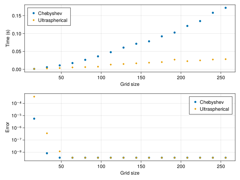
We can see that the ultraspherical method scales linearly with N while the Chebyshev method scales quadratically. The Chebyshev method has a lower error at small grid sizes, but the error converges between the two methods by N=64. At that point, most of the error is due to the time discretization, and it can be decreased further by decreasing the time step.

Spectral methods are really neat ways to solve PDEs accurately without a ton of effort, and the ultraspherical spectral method helps prevent the scaling issues that you get with a pure Chebyshev method. Using a coordinate transformation, it is also really easy to handle the semi-infinte domain that we want for theoretical bottom boundary layer studies. It is pretty straightforward to build an incompressible Navier-Stokes solver in this kind of framework, especially if we use periodic boundary conditions in the horizontal directions. The problem decouples into a set of vertical PDEs like our diffusion equation for each Fourier coefficient. One does have to address the incompressibility condition and the pressure computation, and we might see how that works later. Stay tuned!

You can find the Julia code contained in this file here.