Probabilistic programming in about 100 lines of Julia

using Distributions, LinearAlgebra, Statistics, CairoMakie, Random
Random.seed!(54332187)

The one dependency for our PPL is the Distributions package, which provides a standard interface for working with probability distributions. This is not strictly necessary, but it makes our lives a little easier. Otherwise we would have to write routines for sampling from and computing probability densities for every basic distribution that we want to use in our models. The LinearAlgebra and Statistics standard library modules just provide some functions that will be useful for analyzing our results, and CairoMakie is there to make plots, but none of those are crucial for the PPL implementation. You really can do this entirely in bare Julia.

A strategy for implementing a really simple PPL is write the program in continuation-passing style (CPS) ¹. We augment each probability distribution with a function that has a single argument, the result of sampling from the probability distribution, and returns another distribution, the next distribution in our probabilistic program. If this is a little confusing, it makes more sense in code. First we define a new type for our CPS distributions:

struct LatentDistribution
    f
    s
    d
end

where f is the continuation function, s will be a symbol that we use to name each random variable, and d is the Distribution of the random variable.

The simple probabilistic model \(X \sim \mathcal{N}(0,1)\) now gets written using our LatentDistribution

model = LatentDistribution(X->nothing,:X,Normal(0,1))

Because we only have one variable in our probabilistic model, the continuation function takes the random variable X and outputs nothing, which we will use as a sentinel value to denote the end of our probabilistic program. When you have to write increasingly complex continations, Julia provides a convenient syntax for passing anonymous functions as the first argument to other functions, the do notation:

model = LatentDistribution(:X,Normal(0,1)) do X
    nothing
end

This is identical to the previous model, but slightly easier to read. The benefits become even more clear when we consider a hierarchical model like

This can be written as

model = LatentDistribution(:X,Normal(0,1)) do X
    LatentDistribution(:Y,Normal(X,1)) do Y
        # We don't need to explicitly return nothing
    end
end

Continuation-passing style lets us create an environment in which downstream LatentDistributions know about earlier ones. The distribution for Y can use X as a parameter, because X is passed as an argument to the function that creates Y.

The LatentDistribution objects that we have strung together with continuations don't do anything by themselves. They are, in a sense, a probabilistic program waiting to be run by an interpreter that we have yet to write. We can actually write many different interpreters, depending on the modeling task we want to accomplish. The most basic thing we want to do, however, is to draw random samples from the distribution defined by our probabilistic program.

For the two-level example, we need to do three things

1. Sample X from Normal(0,1)
2. Construct the distribution of Y given the just-sampled value of X, Normal(X,1).
3. Sample Y from that distribution

Sampling X is easy, the desired distribution is stored as the d field of model, so we can call X = rand(model.d). But how do we use this in our probabilistic program? Our continuations come to the rescue. Remember that model.f is the continuation that takes X as a parameter and returns the LatentDistribution for Y. So to sample Y, we would do rand(model.f(rand(model.d)).d), first constructing the LatentDistribution using the continuation and then sampling from the defined distribution.

Of course, in a more complicated probabilistic program, Y would itself be used to define other random variables, so you will want to call its continuation, and so on until you hit a variable whose continuation returns nothing. This calls for some recursion. We define a method

function draw(d::LatentDistribution)
    # Sample from the given distribution
    x = rand(d.d)

    # Call the continuation with the sampled value
    # and draw from that distribution
    draw(d.f(x)) 
end

We also need a method for when we hit nothing

draw(::Nothing) = nothing

We have a problem, though. If you run draw(model) using the model defined above, you will find that it returns nothing. We need to save the random variables that we have sampled. We can do this using a named tuple that associates the symbol of each LatentDistribution (model.s) with its sampled value.

function draw(d::LatentDistribution)
    # Sample from the given distribution
    x = rand(d.d)

    (;d.s => x, # Store the sampled value
     draw(d.f(x))...) # Recurse
end

draw(::Nothing) = (;) # Return an empty named tuple

And now, if we run draw(model), we get something like

(x = -0.2817850808916265, y = 0.6312531437930013)

The next thing we'll need to do is to compute the (log) probability density for a given value sampled from the probabilistic program. For a basic d::Distribution, we do this with logpdf(d,x). For our probabilistic program, we recurse again, combining log probabilities by adding them:

function Distributions.logpdf(d::LatentDistribution,θ)
    # Extract the variable corresponding to the current
    # distribution
    x = θ[d.s]

    # Compute the logpdf of the current variable
    logpdf(d.d,x) +
        # Recurse
        logpdf(d.f(x),θ)
end
Distributions.logpdf(::Nothing,θ) = 0 # Start accumulating probability from 0

This is exactly the same structure as our draw function, except

1. We call logpdf rather than rand.
2. We initialize the recursion with 0 rather than an empty named tuple.
3. We combine the log probabilities by adding rather than concatenating.

The final thing we want to do is statistical inference, estimating the latent variables given the values of observed random variables. We can do this with a new type representing observed variables

struct ObservedDistribution
    f
    s
    d
    y
end

which is identical to LatentDistribution, except it has a field y that gives the value of the observation. We need to implement our sampling and log probability interpreters for ObservedDistribution

function draw(d::ObservedDistribution)
    y = d.y
    (;d.s=>y,draw(d.f(y))...)
end
function Distributions.logpdf(d::ObservedDistribution,θ)
    loglikelihood(d.d,d.y) + logpdf(d.f(d.y),θ)
end

For sampling, we just return the observed value, while for log probability, we use the loglikelihood function from Distributions. This is just like the logpdf function, but computes the log probability for multiple independent and identically distributed observations, which is convenient.

Now we can write a model like

model = LatentDistribution(:X,Normal(0,1.0)) do X
    ObservedDistribution(:Y,Normal(X,1.0),[1.0;-0.2;0.3]) do Y
    end
end

and sampling and log probability calculations will work.

There are many ways to approach inference in probabilistic programs, but we will focus on sampling from the posterior using Markov chain Monte Carlo sampling. Gibbs sampling samples each random variable in turn from its conditional distribution given all of the other distributions. This is only analytically possible for certain probability distributions, so we will instead sample from a different distribution, the proposal distribution, and then use rejection sampling to correct for the fact that the proposal is not necessarily the appropriate conditional distribution. This Metropolis-within-Gibbs sampling is fairly flexible, easy to implement, and lets us design efficient proposals for different parts of our model. The downside is that the proposal design is challenging to automate, so you'll need to do it by hand in our tiny PPL.

First, we will store our proposal distributions in a Dict from the symbols of each random variable to a function that takes a parameter value and returns a Distribution:

proposals = Dict(:X => θ -> Normal(θ.X,0.01))

This way the proposal distributions can depend on the current value of all of the sampled variables. For example, the true conditional probability distribution for our two-level normal model can be found analytically

proposals = Dict(:X => θ -> Normal(1/(1 + length(θ.Y)) * sum(θ.Y),inv(sqrt(1 + length(θ.Y)))))

Now our Gibbs sampling function will take a probabilistic program, the current value of the parameters, and the proposals Dict. For nothing and ObservedDistribution, we don't need to sample anything, so we just return the current parameters, and recurse if we need to.

gibbs(::Nothing,θ,proposals) = θ
gibbs(d::ObservedDistribution,θ,proposals) = gibbs(d.f(d.y),θ,proposals)

For the LatentDistribution, we need to implement the Metropolis-Hastings transition kernel

function gibbs(d::LatentDistribution,θ,proposals)
    # Extract the current variable
    x = θ[d.s]

    # Construct the proposal distribution
    q = proposals[d.s](θ)

    # Sample from the proposal distribution
    x′ = rand(q)
    θ′ = (;θ...,d.s=>x′)

    # Construct the reversed proposal
    q′ = proposals[d.s](θ′)

    # Compute the log acceptance ratio
    α = logpdf(d,θ′) + logpdf(q′,x) - logpdf(d,θ) - logpdf(q,x′)

    # Rejection sampling
    if log(rand()) < α
        # Accept the proposal
        # and recurse
        return gibbs(d.f(x′),θ′,proposals)
    else
        # Reject the proposal
        # and recurse
        return gibbs(d.f(x),θ,proposals)
    end
end

There is one trick here that works even though it is technically wrong. When we call logpdf(d,θ′) and logpdf(d,θ), we only compute the log probability for the variables of the model below the current variable in the chain of continuations. This is okay because the log probability of the other variables can't depend on the current variable. Otherwise we couldn't write the probabilistic program. Since only the current variable changes under the proposal, the log probability of the variables that don't depend on it is just a constant that cancels out in the acceptance ratio, so this works.

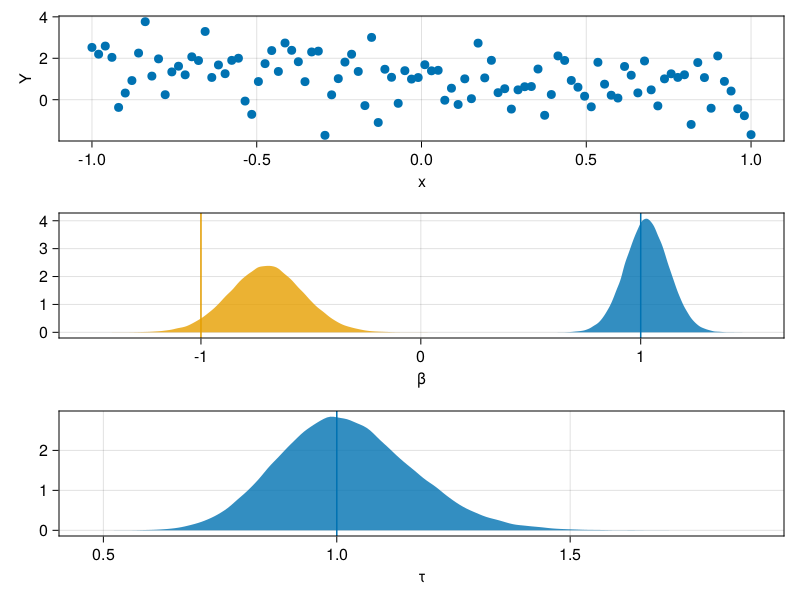
As an example, we will fit the following Bayesian linear regression to some synthetic data

# Generate some synthetic data
N = 100
x = range(-1,1,length=N)
X = [one.(x) x]
β0 = [1.0;-1.0]
σ0 = 1.0

Y = X * β0 .+ σ0 * randn(N)

# Define the model
model = LatentDistribution(:β,MvNormal(Diagonal(ones(2)))) do β
    LatentDistribution(:τ,Gamma(2,1)) do τ
        ObservedDistribution(:Y,MvNormal(X*β,inv(sqrt(τ))),Y) do Y
        end
    end
end

# Define the proposal distributions
proposals = Dict(:β => θ -> MvNormalCanon(θ.τ*X'θ.Y,θ.τ*X'X+I),
                 :τ => θ -> Gamma(2 + length(Y)/2,inv(1 + sum(abs2,θ.Y .- X*θ.β)/2)))

# Draw an initial value from the model
θ0 = draw(model)

# Run 100000 Gibbs steps
θs = accumulate((θ,i)->gibbs(model,θ,proposals),1:100000,init=θ0)

βs = mapreduce(x->x.β,hcat,θs)
τs = map(x->x.τ,θs)

# Plot the results
fig = Figure()
ax1 = Axis(fig[1,1],xlabel="x",ylabel="Y")
scatter!(ax1,x,Y)
ax2 = Axis(fig[2,1],xlabel="β")
density!(ax2,βs[1,:])
density!(ax2,βs[2,:])
vlines!(ax2,[β0[1]])
vlines!(ax2,[β0[2]])
ax3 = Axis(fig[3,1],xlabel="τ")
density!(ax3,τs)
vlines!(ax3,[inv(σ0^2)])
save("linear_regression.png",fig)

So there you have a rudimentary probabilistic programming language in only a few lines of Julia. Drawing random samples, computing log probabilities and Metropolis-within-Gibbs sampling from the posterior distribution are all just different interpreters of the same probabilistic program. We could conceivably implement other inference algorithms like Hamiltonian Monte Carlo or variational inference just by walking down the chain of continuations and accumulating the necessary information at each step.

There are many limitations to our tiny PPL. We have to write out the continuations explicitly in the do notation syntax. It doesn't support the stochastic control flow structures that distinguish true probabilistic programs from basic probabilistic models. It probably also doesn't perform very well with complicated models and big data.

I learned a lot from the following three references, which I highly recommend if you are interested in the inner workings of PPLs.

• Noah D. Goodman and Andreas Stuhlmüller. The Design and Implementation of Probabilistic Programming Languages. http://dippl.org/
• Jan-Willem van de Meent et al. An Introduction to Probabilistic Programming. https://arxiv.org/abs/1809.10756
• Jonathan Law and Darren Wilkinson. Functional probabilistic programming for scalable Bayesian modelling. https://arxiv.org/abs/1908.02062