Random maps with spatially dependent Pitman-Yor processes

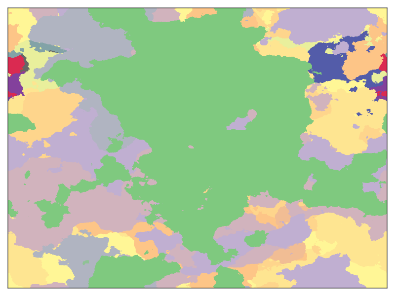
Gaussian processes are powerful tools for modeling spatially varying fields like sea surface temperature or sand ripple elevation. But what can you do if you want a model for discrete-valued fields like a land cover classification? There are many approaches that you could use for this problem, but I particularly like the maps you can generate using spatially dependent Pitman-Yor processes (Sudderth and Jordan 2008).

A Pitman-Yor process is a generalization of the Dirichlet process. Both are probability distributions over probability distributions in a sense that is quite tricky to understand, but which is very useful in developing nonparametric Bayesian models for data: you can use a Dirichlet/Pitman-Yor prior for an unknown probability distribution and then learn the distribution from your data.

Another way of looking at these processes is that they provide distributions over infinite partitions of the interval \([0,1]\). This is often called the "stick-breaking" construction of the Dirichlet process, and it works like this. Imagine we have a stick with a unit length. We first break off a randomly sized fraction of the stick, \(v_1\). This is the first segment of our partition with length \(p_1 = v_1\). Now we take the remaining stick, which has a length \(1 - v_1\), and we break off another piece that is a fraction, \(v_2\), of the remaining length. This piece is our second segment, and it has a length of \(p_2 = v_2 (1 - v_1)\). We repeat this process an infinite number of times, so that the $k$-th segment has a length \(p_k = v_k \prod_{i=1}^{k-1} (1 - v_k)\), and the segments all add up to the length of the original stick \(\sum_{k=1}^{\infty} p_k = 1\).

The difference between the Dirichlet process and the Pitman-Yor process is simply in the distribution of the fractions, \(v_k\). The Dirichlet process has each fraction distributed by a \(\text{Beta}(1,\alpha)\) distribution while the Pitman-Yor process has

\[ v_k \sim \text{Beta}(1 - \beta,\alpha + k \beta) \]

so that the distribution changes with \(k\). When \(\beta = 0\), this is just the Dirichlet process while higher values of \(\beta\) result in a distribution with heavier tails than the Dirichlet process.

For our Pitman-Yor process maps, we only need to sample the fractions, \(v_k\), which we can do easily in Julia using Distributions.jl to sample from the Beta distribution

function sample_py_fractions(α,β,K)
  v = zeros(K)
  for k in 1:K
      v[k] = rand(Beta(1 - β, α + k * β))
  end
  v
end

Note that even though the partition formally has an infinite number of segments, we only sample the first \(K\) fractions. One interpretation of the Dirichlet process is as a mixture model with an infinite number of components. The partition lengths, \(p_k\), are the relative frequencies of each class: \(p_1\) percent of your data will come from class 1, \(p_2\) come from class 2, and so on. Since \(p_k\) is always smaller than \(p_{k-1}\), only a finite number of classes will have a meaningful probability of being drawn, even though the model theoretically represents an infinite number of classes. As long as \(K\) is high enough that we don't hit that threshold, it is okay to only think about the first \(K\) classes.

In this classification model, it turns out that the stick-breaking fraction \(v_k\) is the conditional probability of assigning a data point to class \(k\) given that all the classes with indices less that \(k\) have been rejected. So we can think about generating class assignments by first choosing class 1 with probability \(v_1\). If we don't choose class one then we choose class 2 with probability \(v_2\), and so on, until all of our data points are assigned to classes. In code, this process looks something like

function generate_classes(v,N)
    z = zeros(Int,N)
    for i in 1:N
        k = 1
        while (k <= length(v)) && (rand() > v[k])
            k += 1
        end
        z[i] = k
    end
    z
end

The insight that allows Sudderth and Jordan to create spatially dependent Pitman-Yor processes is that instead of drawing uniform random variables and checking whether they are less than the stick-breaking fraction, we can draw random variables from a different distribution, apply the cumulative distribution function for that distribution to the random variable and compare that value to the stick-breaking fraction. This is the same idea behind inverse transform sampling, which lets you convert uniformly distributed random variables into arbitrarily distributed variables provided that you know the (inverse) cumulative distribution function.

In particular, we can choose standard normal random variables and apply the CDF of the normal distribution to sample from the same distribution of classes. Furthermore, instead of drawing independent samples, they can have correlations across the data points, as long as the marginal distributions are standard normal. It is important to note that the correlations are across data points (the index \(i\) in the above code) not the classes. Those still need to be independent to get the class proportions correct.

Gaussian processes are just normally distributed random variables with spatial correlations, so we can build spatially dependent Pitman-Yor processes by first drawing \(K\) independent realizations of Gaussian processes over our region of interest, drawing stick-breaking fractions as above, and then applying our classification scheme for each point in space.

There are a lot of details to sampling from Gaussian processes, so we won't look into them in great detail here. Instead we will just use the following function that generates random fields on regular grids using fast Fourier transforms.

function generate_field(k0,ν,Nx,Ny,B)
  kx = FFTW.rfftfreq(Nx)
  ky = FFTW.fftfreq(Ny)
  k2 = abs2.(kx) .+ abs2.(ky')
  v = inv(sqrt(π/ν)) * (k0^ν) .* (abs2(k0) .+ k2).^(-(ν+1)/2)
  irfft(v .* rfft(randn(Nx,Ny,B),(1,2)),Nx,(1,2))
end

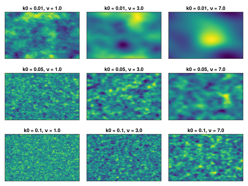
The parameter \(k_0\) sets the correlation length of the field: higher \(k_0\) corresponds to shorter correlation lengths, and the parameter \(\nu\) controls the smoothness of the field, with higher \(\nu\) giving smoother fields. The following figure illustrates some random fields as shown in the following figure

k0 = [0.01;0.05;0.1]
ν  = [1.0;3.0;7.0]

fields = [generate_field(k0,ν,256,256,1)[:,:,1] for k0 in k0, ν in ν]
fig = Figure()
for j in 1:3
    for i in 1:3
        ax = Axis(fig[i,j],title="k0 = $(k0[i]), ν = $(ν[j])")
        heatmap!(ax,fields[i,j])
        hidedecorations!(ax)
    end
end

save("patchwork-fields.png",fig)

Finally we just need to modify generate_classes so that it uses the random fields as input to generate the classes.

Φi(v) = -erfcinv(2v) * sqrt(2)
function classify_fields(u,v)
  z = zeros(Int,size(u,1),size(u,2))
  for j in 1:size(u,2)
      for i in 1:size(u,1)
          acc = false
          k = 1
          while (k < size(u,3)) && (u[i,j,k] >= Φi(v[k]))
              k += 1
          end
          z[i,j] = k
      end
  end
  z
end

Note that we defined the function Φi(v) which is the inverse of the standard normal cumulative distribution function.

We can wrap all of this together in a function to generate a map

function generate_map(α,β,k0,ν,Nx,Ny,K)
    v = sample_py_fractions(α,β,K)
    u = generate_field(k0,ν,Nx,Ny,K)
    classify_fields(u,v)
end

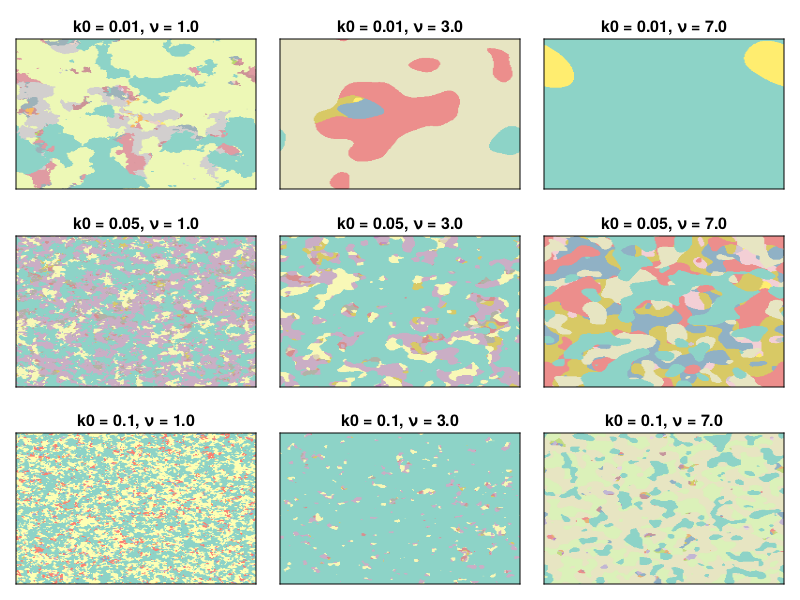
and make some maps

k0 = [0.01;0.05;0.1]
ν  = [1.0;3.0;7.0]

maps = [generate_map(1.0,0.0,k0,ν,256,256,32) for k0 in k0, ν in ν]

fig = Figure()
for j in 1:3
    for i in 1:3
        ax = Axis(fig[i,j],title="k0 = $(k0[i]), ν = $(ν[j])")
        heatmap!(ax,maps[i,j],colormap=:Set3_12)
        hidedecorations!(ax)
    end
end

save("patchwork-maps.png",fig)